Introduction to normal distribution

From scratch

Today’s post is about the most popular distribution ever: The normal distribution.

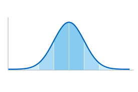
The normal distribution, also known as the Gaussian distribution, was proposed by the German mathematician Carl Friedrich Gauss in the 19th century. Gauss observed that a large number of phenomena in nature, such as the height of people, the weight of objects, errors in measurements, etc., follow a distribution pattern that resembles a bell, with most values clustered near the average and fewer values moving away from the average.

The normal distribution is characterized by having a mean and a standard deviation. The mean is the central value of the distribution, while the standard deviation measures the variability of the data. The shape of the normal distribution is symmetrical and is described by a mathematical function known as the probability density function, which measures the probability that a certain event occurs.

This distribution is one of the most common probability distributions due to several reasons:

It is a continuous distribution, meaning that it has a continuous curve and an infinite number of possible values. It is a bell-shaped distribution, with a peak in the centre and symmetry on both sides of the peak. It is a well-known and well-studied probability distribution, with a large amount of theory and statistical tables available.

However, the normal distribution has some limitations:

-It does not fit well with data that have a highly skewed or asymmetric distribution.

-It cannot be used to describe discrete variables.

-It cannot be used to describe variables that have a finite range, such as categorical variables.

To sum up, let's take a very simple example of how the daily return of a stock can be a normally distributed random variable: Suppose you have a stock whose average historical return is 0.02 (2%) and a standard deviation of 0.03 (3%). Then, you can assume that the daily stock return follows a normal distribution with a mean of 0.02 and a standard deviation of 0.03. This means that 68% of the time, the daily stock return will be between -0.01 and 0.05 (2%-3% and 2%+3% respectively).

In addition, the normal distribution can be used to calculate probabilities associated with certain levels of performance. For example, one can calculate the probability that the daily stock return will be greater than 0.03 (3%). This could be useful to establish an investment strategy or to calculate the Value at Risk of a portfolio.