Experimenting with the essentials of econometrics using R

First of many, hopefully

In order to see the value of data, let’s quantify the extent of marital status in the U.S. Data has been collected from email queries of citizens to public offices (libraries, police, registry), whereby citizens were asked in a survey to provide the relevant information. In particular, the survey includes data on 1) a person’s marital status — “married”, “single”, “divorced”, and 2) data on how many hours it takes for a public office to respond.

We want to estimate the effect of marital status (i.e. a dummy that equals one if a person isn’t in a relationship — either single or divorced— and zero if the person is married) on the response time to an email. Our goal is to figure out if married people (families) have more priority than single people in public services.

Dummy variables are useful to include qualitative information into empirical analysis. In order to estimate this effect we could use the following regression equation: Yi= ß0 + ß1 Xi + Ui, where Xi is the binary variable ( Xi= 1 if the person isn’t in a relationship and Xi= 0 if the person is married), Yi quantifies the response time to an email, and Ui is the error term. Notice that we are not in the case in which we have a binary dependent variable ( i.e. does a consumer buy a product or not).

We are interested in the parameter ß1, which is the slope of the regression line but also the difference in means of the two groups:

ß1= E(Yi/Xi=1) — E( Yi/Xi=0) By estimating ß1 we can quantify up to what extent there is an effect on being part of a marital status that affects the time of the response of an email.

On the other hand, we can also discuss the random sampling assumption and the conditional independence assumption (E(u|X) = 0).

The Conditional independence assumption is fulfilled since there are no external factors (u) that could affect the marital status of someone (X) and the same occurs with the random sampling assumption. The data is collected from the same population, then it is identically distributed, and we assume the surveys were taken randomly, so the values are also independently distributed. Since these assumptions are fulfilled, we can get an estimate very close to the actual one of population. If not, the result could be biased by the u, thus the sampling 1 has 0 approximation to the real 1.

To solve this, an ideal experiment for this case would be one based on surveys conducted randomly on people of both different marital statuses (single or not single) and then compare the average number of hours it took to be answered by the public office, thus arriving at the true result of whether there is discrimination in the public sector.

We can use R to produce a table of summary statistics (number of observations, mean, sd, median, min, max, number of missing observations) for the variables reply, complexity,cordial_reply, length_reply and marital status, referring to some characteristics of the emails.

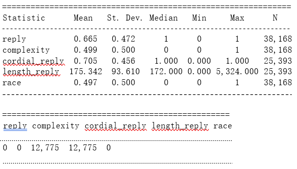
As we can observe we have, on the one hand, the summary statistics regarding the variables that we are interested in a number of observations, mean, sd, median, min, max) and, on the other hand, the number of missing information. Finally, according to the information regarding the mean of the variables, we can deduce: There are more emails that received a reply than emails that have not, as the dummy variable mean was over 0,5. Notice that we can´t say that 66.5% of the email has been answered, because we are not talking about a continuous variable, but a dummy variable.

There are more complex emails than no complex emails, as the dummy variable was over 0,5. Notice that we can´t say that 70.5% of the emails are cordial because we are not talking about a continuous variable, but a dummy variable.

There are more cordial replies than no cordial replies, as the dummy variable was over 0,5. Notice that we can´t say that 44.9% of the emails are complex because we are not talking about a continuous variable, but a dummy variable.

The mean for the length of replies is 175.345 words per email. There are more singles than married, as the dummy variable was under 0,5. Notice that we can´t say that 49.7% of the emails are sent by married, because we are not talking about a continuous variable, but a dummy variable. It is important to take into account that the mean is very close to 50% as the aim of the project is to a quantifies the extent of marital discrimination in local public services in the U.S, therefore it is important that there is an equilibrium between both variables.

Another idea is to run t-tests comparing the difference in means between singles and married for the following variables: reply, cordial_reply, length_reply, delay_reply. The results of the t-tests are presented in a table that shows the following: each row is a variable; columns: mean of the variable for singles, mean of variable for marrieds, the difference in means between singles and married, a p-value of t-test. We can interpret the findings regarding the magnitude and statistical significance:

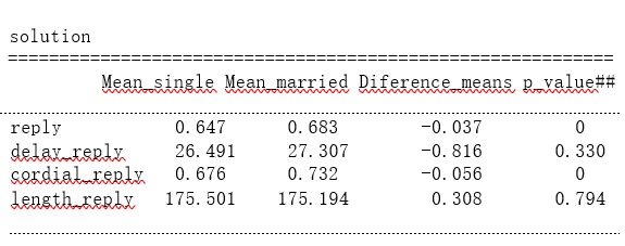
With this input, we obtain information regarding the mean of the variable for singles, the mean of variable for marrieds, the difference in means between singles and married, a p-value of the t-test.

According to the following table, and taking into account that the reference group is x= 0, this is the white group, we can observe that: Although more emails were replied on average to the married group, it is also true that the delay of the reply was larger for them, in detail, 0,816 hours more on average. Additionally, the length of the reply to the email is on average larger for single than for married senders, in detail, 0.308 more words on average. Nevertheless, there were more cordial replies on average for the married group than for the single group. Finally, it is key to understand that as the p-value of reply and cordial_reply are so low, we have approximated it too but, in fact, they are 3.27e-14 for reply and 1.25e-22 for cordial_reply.

Finally, let’s regress the dummy reply on the dummy marital status. We may interpret the coefficients of the slope and intercept, comment on statistical significance, and compare your results to those above:

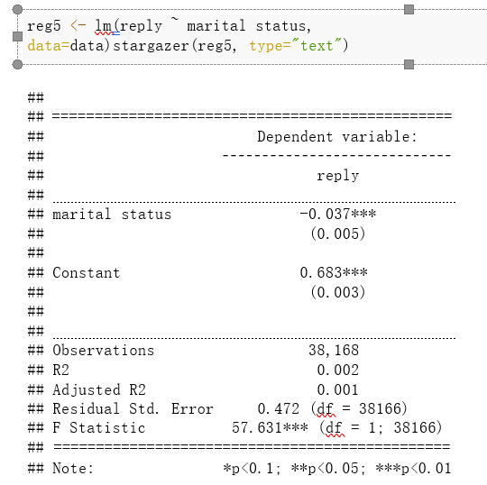
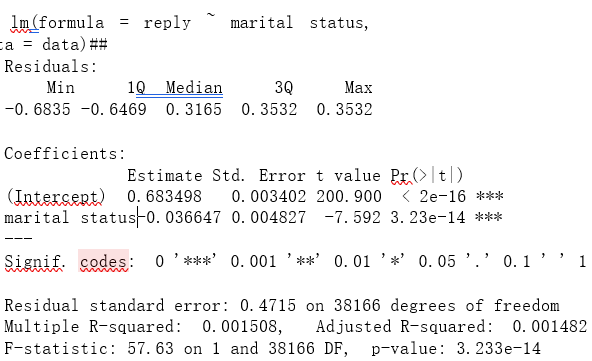
In this regression line we have a negative intercept. It means that if the marital status is married (0) the reply would be negative, which it makes no sense, it is not possible to have negative replies. Then the 1 is 0.683, due to being less than 1, it shows that a change from 0 to 1 in marital status would mean a change in the probability of receiving a reply of 68.3%. Eventually, we have a very strong statistical significance because the p-value is a very small number, meaning that the difference in replies received between marital statuses is statistically significant.